| What
is Driving the Gold Price?
An Empirical Investigation
BY Craig Graham Tennant (1)

 Abstract
 ince the 1980’s, the gold price has been on a slow downward
trend reaching a low in April 2001 of $250 an ounce before
commencing an upward run to a peak of $720 in May 2006. It
is essential to understand what is driving the gold price.
This paper uses simple statistical and econometric analysis
for the period January 1995 to November 2005. Amongst other
things, it is established that a statistically significant
negative relationship exists between the gold price and the
US dollar exchange and gold leasing rates, and that a statistically
significant positive relationship exits between the gold price
and world income. Gold’s expected relation with inflation
does not hold over the period.
Keywords: gold market, price determination,
macro-determinants, commodity markets, semilog model, gold
lease rate, US dollar, inflation, world income
GOLD IS A PRECIOUS METAL WHICH occurs naturally
in various ore formations in the earth’s crust. The
recovery of gold from gold bearing ore occurs in most instances
where the concentration of gold in mineralized(2)
ore bodies is sufficient to support the economic exploitation
by mining and recovery of gold bearing ore to the physical
form of gold metal. The production of gold is therefore the
result of an economic activity which has a profit motive.
Any decision to produce gold from the activity of mining to
refining would be determined by the price of gold and the
relative cost of such activities. The secondary sources of
gold supply are firstly, the supply of gold from gold scrap,
which is primarily obtained from gold in scrap fabricated
products such as jewellery, industrial components, electrical
contacts, and coins (Gold Fields Mineral Services 1991:26)
and secondly, from official bullion(3)
sales by central banks and financial institutions like the
International Bank of Settlement. The leasing of gold is largely
influenced by the gold leasing rate. The amount of gold that
is supplied to the market will thus be affected by changes
in these four activities.
The demand for gold can broadly be divided
into two categories, firstly, a view of gold, based on its
beauty, rarity, physical characteristics or intrinsic value,
which give rise to the “use demand”. Here gold
is used in industry and the production of, jewellery, medals,
coins, and electrical contacts, and in the field of dentistry.
Secondly, the view that gold is a store of value based on
the assumptions that gold is a hedge, and provides protection
to wealth when other assets are losing their value. This gives
rise to the “asset demand” for gold, the use of
gold bullion by central banks, fund managers, and individual
investors.
Gold has four unique attributes that set
it apart from other commodities: firstly, gold is a noble
metal which effectively makes it indestructible, meaning that
it is not subject to the weathers of erosion and decay over
time. Secondly, gold has a very high value to volume ratio.
Thirdly, gold is perfectly homogeneous, and is traded continuously
in well organised markets; and fourthly, annual supply in
the typical case of 2004, of about 4100 tonnes (The Department
of Minerals and Energy 2004:39), is dwarfed by the above ground
global stock of gold, estimated at 145,000 tonnes by Lawrence
(2003:3), which includes the worlds total above ground stock
of gold including total financial reserves and all privately
held jewellery, bullion and coins.
Since the demise of the Bretton Woods system
in 1971, the gold price was allowed to fluctuate freely in
the market and has since been subjected to the law of supply
and demand as any other commodity is (Evans, 2003:4). As a
result, it is thus expected that a sudden and unexpected rise
in the demand for gold, which is not matched by an equivalent
rise in the supply of gold, would cause upward pressure on
the market price of the metal.
One of the criticisms of the supply and demand
hypothesis, in determining the fair value of gold, which is
unique to the gold market, is the fact that large supplies
of above ground inventory are relatively liquid and likely
to dampen any spike in demand. One version of this argument
is by Lawrence (2003) who theorises that the supply of gold
is perfectly elastic. Much of the worlds stock of gold is
available in a form that can easily enter the market; often
the financial position of individuals supports the selling
of gold back into the market if the price is right. There
are also means for gold held by central banks and the IMF
to re-enter the market via sophisticated gold leasing mechanisms.
Faugère and Van Erlach (2005:3) mention
that “assessing the fair value of gold largely remains
a mystery in finance.” This paper suggests a fresh look
at this unique metal, by exploring the determinants of the
gold price, and will attempt to explain what is driving the
gold price? The broad objective is to determine empirically
the factors that are responsible for driving the gold price
during the period January 1995 to November 2005. The focus
will be on factors believed to be the main drivers of demand
for gold. Variables analysed were determined by the availability
of data and those thought to be relevant to the gold market.
The paper is organised as follows. Section 1 addresses the
context and importance of the research, and outlines its goals.
Section 2 summarises previous academic literature on the issue
of non-renewable resources and the gold market. Section 3
sets out the research methodology adopted, model specifications,
and data issues, whilst section 4 presents the results and
estimates for the gold demand function. These results are
discussed and concluded in section 5.
1. Context
and Goals
A large upward run in the gold price began in the early 1970’s
and ended in the mid 1980’s at a peak of $835 an ounce.
Prior to 1971 the monetary system called the Gold Standard
or Bretton Woods accord was in effect. The US dollar was expressed
in terms of a gold price fixed at $35 an ounce. The gold market
then entered a seventeen year period(4)
of falling gold prices from the mid 1980’s to its lowest
level in April 2001 at a price of $250 an ounce. Since then,
gold has been on a steady upward run where prices have been
as high as $720 in the first quarter of 2006, levels not seen
in the past 26 years (Dorsch, 2006). This price movement,
as well as the incredible rate of price increases, especially
from mid 2005, have generated a lot of journalistic interest
and are not only important in a global, but also a South African
context since South Africa has consistently been the world’s
leading gold producer for the last 120 years (Roger Baxter
the Chamber of Mines Chief Economists, interview with Ryan,
2006:79). Within a South African context a rise in the gold
price has an important impact on employment levels, the value
of the SARB reserve assets, the value of the export component
on the Balance of Payments, and the value of the Rand, although
the relationship with the Rand is controversial (Waggoner,
2005).
This research is intended to be a re-look
at the driving forces of the gold price. Since the last great
Bull Run in the gold price during the early 1980’s economic
conditions have changed, new influences have evolved, economic
structures have grown, and new orthodoxies have been established.
The Cold War is over and the Berlin wall has fallen. The world
has become increasingly a global village, and the impact of
globalisation has increased trade and capital flows between
nations, beyond anything ever imagined in the 1980’s.
The global impact of India and especially China over the last
decade as major metal and raw material consumers was never
considered up until recent times, as well as a rapid rise
in the middle class and a relaxing in economic barriers (GoldOrg,
2006). Generally more currencies around the world have become
free floating and determined by the market, there is also
the new phenomenon of the Euro currency being regarded as
an international currency (Keyfitz, 2004).
By exploring the determinants of the gold
price, this paper can bring new explanations to the question
of, what is driving the gold price. This is of interest to
the business community, government, the mining industry, bullion
banks and investors. This research thus aims to shed some
light on a select number of variables that have shown both
theoretical and empirical links with the demand for gold,
and which the author believes are responsible for driving
the gold price during the period 1995 to 2005. This paper
will thus employ simple statistical and econometric analysis
to estimate a demand function for gold. Research questions
addressed are; to determine the specific relationships between
the following variables and the gold price.
- Determine the extent of the relationship between the
gold price and world inflation index, and inflation in
the United States.
- Determine the extent of the relationship between the
gold price and the nominal broad dollar index.
- Determine the extent of the relationship between the
gold price and the gold leasing rate.
- Determine the extent of the relationship between the
gold price and world income.
2. Literature
Review
There are a number of factors that impact
the gold price; the extent of the impact can be established
empirically. One branch of economics that deals with the topic
of the gold market is the economics of non-renewable resources.
The theory originates with the pioneering work of Harold Hotelling
who studied the optimal depletion of resources. Hotelling
was driven by his concern for the adequacy of the world’s
natural resource base. The mineral resources industry is unique
from other industries in that it is “… an industry
in which the indefinite maintenance of a steady rate of production
is a physical impossibility…” by Hotelling(1931:139)
in Devarajan and Fisher(1981:66). The first approach, the
“Hotelling Rule” was established which states
that the price of an exhaustible resource must grow at a rate
equal to the rate of interest, both along an efficient extraction
path and in competitive resource industry equilibrium. By
saying that the net price of a non-renewable resource, assuming
extraction costs are nil, must rise in successive years by
the rate of interest implies that the price of gold, for example,
must rise by the rate of interest as well (Deverjan and Fisher
1981:66).
A numerical example that has been modified
from Salant (1995:98) and again illustrated in Solow (1974:3)
shows this condition well. With an interest rate of ten percent
and the net price per ounce of gold at $300 an ounce, if the
gold price is expected to be at a price below $330 in the
next period, it pays to extract more gold in the current year,
because the income will earn ten percent interest. This is
because no asset holder would wish to hold resources in the
ground and all production would be shifted to the current
period. On the other hand, if the net price is expected to
be above $330 and thus grow faster than the rate of interest,
gold miners will have no incentive to mine gold in the current
period. By delaying production suppliers place pressure on
the gold price to rise. In this case, resource deposits left
in the ground would be a superior way of holding wealth. From
this analysis, it is observed that there is a natural tendency
for the net price of exhaustible mineral deposits to appreciate
at the rate equal to the rate of interest prevalent in the
economy, maintained by producers adjusting their production
based on the expected future gold price.
Keyfitz, 2004; Sjaastad and Scacciavillani,
1996; Capie, Mills, and Wood, 2004 established that fluctuations
in exchange rates have a significant effect on the gold price.
The Sjaastad and Scacciavillani (1996:880) study is based
on the same assumptions, used by Keyfitz (2004), that global
markets clear and the law of one price holds. Sjaastad and
Scacciavillani (1996:884) find that, for the period 1982-1990,
“European countries heavily dominate the international
market for gold and hence movements in European exchange rates
against the US dollar impact heavily on the dollar price of
gold. Capie, Mills, and Wood (2004) examine the relationship
between gold, and exchange rates of various currencies against
the dollar and how well gold has performed as a hedge, with
respect to exchange rate fluctuations. This paper reveals
that there is a negative correlation, which is not statistically
significant, between the gold price and the dollar exchange
rate.
Ghosh, Levin, Macmillan, and Wright (2002)
examine the short and long term determinants of the gold price.
Their main findings reveal that gold is mostly an inflationary
hedge in the long run. Furthermore they state that the short
run price fluctuations in the gold price are due to changes
in the real interest rate, US dollar exchange rate, and the
leasing of bullion by central banks, all of which according
to Ghosh et al. (2002:1), “…can disturb this equilibrium
relationship and generate short-run price volatility.”
An exception to the above findings, Lawrence
(2003:6) studies the lack of correlation between the return
on gold and the return on financial assets such as equities.
He attributes this difference to his “hard line”
hypothesis that states, “the impact of cyclical demand
– using as proxies GDP, inflation, nominal and real
interest rates, and the term structure of interest rates –
on returns on gold, is negligible, in contrast to the impact
of cyclical demand on other commodities and financial assets.”
Lawrence (2003:5) concludes that, “There is no statistically
significant correlation between returns on gold(5)
and changes in macroeconomic variables, such as GDP, inflation
and interest rates.”
Faugère and Van Erlach (2005:2) view
gold as a global real store of wealth or as a hedging tool
against inflation and the fall in value of other investments.
Gold has become more and more a global investment vehicle
and is therefore subject to a minimum required yield. Although
Lawrence (2003:7) specifically mentions that there is no correlation
between returns on gold and those of equities and bonds. Faugère
and Van Erlach (2005:6) believe, “A preliminary investigation
of the price of gold reveals a non-trivial connection between
real gold prices and the US stock market.” To be considered
a global real store of value it must maintain real purchasing
power over time even though gold does not provide actual earnings.
Gold does not need to produce the same return as other assets,
but rather to maintain its store of value. This is ensured
by the amount of capital flows into gold, which according
to Faugère and Van Erlach (2005:7), is “dictated
by changes in the minimum expected return achieved by other
asset classes.” Therefore movements in the gold price
are as a result of the “precautionary demand for gold.”
Gold must vary directly with the global required yield and
current expected inflation for it to fulfil its purpose of
providing investors with a minimum after tax return.
3. Research
Methodology and Data Issues
Time series data collected for this study
consists of monthly data from January 1995 to November 2005.
Firstly, the gold price (Gp) was obtained from the website
(www.EconStat.com); the monthly spot average price is quoted
in US dollars per troy ounce(6) . Gold
is traded around the world and always quoted in US dollars
and thus considered homogenous. Secondly, the effect of exchange
rates on the gold price will be considered using a Nominal
Broad dollar Index (US$ex) which will provide a good indicator
of the strength and weakness of the dollar over the period.
The index was obtained from the Federal Reserve and is a weighted
average of the foreign exchange values of the US dollar against
the currencies of a large group of major trading partners.
Thirdly, as a proxy for inflation in the United States, a
monthly US Consumer Price Index (USinf) for all items, city
average and not seasonally adjusted was used, obtained from
(www.EconStat.com). This was then converted into month-on-month
inflation data by calculating the monthly percentage change
in the index. Fourthly, the World Inflation Index (Winf) was
obtained from the International Financial Statistics Database;
this was converted into month-on-month inflation data using
the same method(7) . Fifthly, as a measure
of world income (WorldY), a proxy was used. A number of studies
have used world income as an explanatory variable for the
price of gold. Levin and Wright (2006) used world GDP which
was interpolated to obtain a monthly data series as a proxy
for world income(8). However the use
of world income (WorldY), as a possible variable in explaining
the gold price in this sense is limited. The limitations of
using an interpolated percentage change in world GDP growth
rate, as a proxy for world income, is firstly as a result
of the very interpolation process which makes this data useful.
Gujarati (2003:447) indicates the limitations of data massaging
techniques, stating that such data might possess a systematic
pattern that was not originally in the data, and may introduce
autocorrelation. The second limitation of using the percentage
change in world GDP as a proxy for world income is one of
economic theory. It is expected that a positive relationship
exists between, income and the demand for a good. At first
glance, an increase in income will result in an increase in
demand for gold through an increase in the demand for jewellery,
commemorative gold coins, and for gold as an investment good
etc, and hence an increase in the price of gold. However this
relationship will be difficult to interpret because in the
above analogy, we are actually concerned with changes in “real”
income. This proxy for world income (WorldY) does not take
into account the effects of world inflation over the period
and thus in effect can be seen as a “nominal”
change in world income. For example, if world income and world
inflation are shown to rise together, then in effect there
is no change in “real” world income which would
be the variable normally used to measure changes in income
with changes in demand. Thus the variable world income (WorldY)
is misleading in the sense that it was developed as a proxy
for world income and can only be considered in “nominal”
terms. Based on suggestions and the obvious problems just
mentioned, this paper will make use of industrial production
for all developed countries as a proxy for world income .
This data was obtained from the International Financial Statistics
Database and has been used in various studies as a proxy for
world income. Lastly, the daily London Bullion Market Association
(LBMA) Mean Gold Lease Rate (Glease) was obtained for the
period under investigation. This was converted into monthly
data by taking the average rates over each month for the period
of the sample(9) .
The time period January 1995 to November
2005 as seen in Figure 1, was chosen specifically because
it depicts an interesting period in the gold market, namely
the steady downward trend in the gold price from the 1980’s
to its lowest point in April 2001 at around $250 an ounce,
followed by a steady upward trend that started in late 2001
and accelerated towards the last quarter of 2005. Dorsch (2006:1)
believes that this turning point has constituted the beginning
of what he terms a “Commodity Super Cycle” which
essentially means that world commodity markets are at the
beginning of a long run upward cycle. Dorsch has observed
the Reuters Jeffries Commodity Price Index(10)
rise by 91% over the last 4 years from the end of 2002 to
the beginning of 2006. It is hypothesised that the variables
stipulated in this paper are responsible for driving the gold
price over this period.
3.1 Graphical
Analysis
The analysis was carried out through simple visual plots of
the data. From this visual analysis trends and correlations
can be seen. The advantage of this approach is that it is
easy to use and thus widely utilized. Time series data poses
a number of challenges in econometric analysis. According
to Gujarati (2003:807), a graphical plot of the data can give
an indication about the likely nature of the time series;
however this study will rely on more formal tests of stationarity.
A number of statistical tests may be used, the most popular
is based on the unit root test developed by Dickey and Fuller
(1979, 1981) (Muscatelli and Hurn, 1992:5).
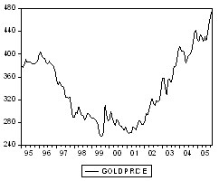
Figure 1. Gold’s average monthly spot price (US
dollars an ounce).
Figure 1 (Gp) plots the gold price which
trends downwards from 1995 to 2001. It can be seen that after
2001, the gold price rises rapidly to the end of 2005.
3.1a. Gold
Loans
One of the unique characteristics of the gold
market is that there are large inventories of above ground
stock. Table 1, shows the official sector gold holdings for
2004. The table shows central bank accumulated gold lending
in tonnes for the period 2001 to 2005. Together Europe and
North America accounted for approximately 70% of official
global Central Bank bullion reserves. The worlds total financial
reserves of gold which includes all official Central Bank
bullion holdings as well as significant holdings of global
financial institutions like the IMF, accounts for approximately
25% of the worlds mined gold. At a value of $550 oz this would
amount to approximately R4.261 trillion(11)
. The gold loan market is used for two main purposes; firstly,
as a source of financing. This is attractive because often
the interest rate on loans is much higher than the gold leasing
rate. In this case, companies borrow gold from the central
bank, sell it on the spot market and use the proceeds to pay
off existing debt or to finance new mining projects (Gold
Fields Mineral Services 1991:28). Secondly, gold producers,
via the same gold lending market can supply their customers
by leasing gold, or by extracting it from their mining activities
(Ghosh, Levin, Macmillan, and Wright, 2002:5). The gold leasing
rate is largely responsible for the quantity of above ground
stock re-entering the gold market. An official definition
from Gold Fields Mineral Services (2005:10) states the gold
lease rate is, “The cost of borrowing or return from
lending gold, the daily level of which reflects the supply
and demand for metal in the lending market.”
Table 1. Official sector holding (2004);
Central bank lending, (2001-2004)
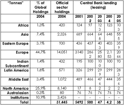
Note: Data obtained from Virtual Metals Research Consulting,
2005:31
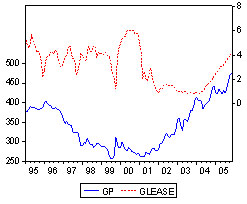
Figure 2 Gold Lease Rate and corresponding Gold Price
(US dollars an ounce).
Economic theory suggests that a high gold
leasing rate, as seen in 2000 and 2001, depresses the gold
price by firstly increasing the supply offered to the market
by central banks, and secondly by dampening the demand for
such gold (Ghosh, Levin, Macmillan, and Wright, 2002:20).
A negative relationship is expected between the gold price
and the gold lease rate. Figure 2 reveals that this negative
relationship holds from 2000 to 2004; however the relationship
becomes ambiguous over the period 1995 to 1999 as well as
in 2005. The relationship will become clearer when statistical
analysis is done.
3.1b. US Inflation

Figure 3 US month-to-month Inflation rate and corresponding
Gold Price (US dollars an ounce).
A state of continued and sustained rising
prices over a time period or else known as the inflation rate,
can be viewed as the opportunity cost of holding money as
apposed to real assets. Figure 3 plots the US inflation rate
and the gold price on the same axes. The month-to-month inflation
rate remains above the zero percent rate indicating an accumulated,
increasing rate of inflation over the period, however the
inflation rate becomes increasingly volatile from 1999 to
2005. As the rate of inflation increases, the purchasing power
of money diminishes, and at the same time the value of real
assets remain the same. To clarify this point an example has
been taken from Ghosh, Levin, Macmillan, and Wright (2002:2)
which states that:
“In 1895 the price of gold was $20.7 per ounce, or about
$379 in 1995 dollars, while in 1995 it was $387—virtually
no change in the real value of gold over a one-hundred year
period. Fitting a trend line indicates that the real price
of gold increases on average by only 0.3 per cent per year
in this hundred-year period.”
This view of gold as an effective hedge against
inflation over the long run gives gold its “store of
value” characteristic. A positive relationship between
US inflation and the gold price is therefore expected. There
does appear to be large deviations between the gold price
and the US month-to-month inflation rate which corresponds
with Ghosh, Levin, Macmillan, and Wright (2002) hypothesis
that gold is only an inflation hedge over the long-run.
3.1c. World
Inflation

Figure 4.World month-to-month Inflation rate and corresponding
Gold Price (US dollars an ounce).
Figure 4 plots the month-to-month world inflation
rate (Winf). It suggests that a high gold price is synonymous
with a high inflation rate between 1995 and 1999, however
this positive relationship does not hold between 2001 and
2005. This confirms the findings of Ghosh, Levin, Macmillan,
and Wright (2002), that gold is only an inflation hedge in
the long run, and that short term fluctuations are largely
due to exchange rate, leasing rate, and interest rate changes.
3.1d. US Nominal
Broad Dollar Index
The Nominal Broad Dollar Index rate appreciated
over the period 1995 to mid 1998, moving from 90 to 120 points.
The dollar held its strength at this level until 2000 before
it climbed to a high of almost 130 points in late 2001. Since
late 2001 the dollar index has depreciated to just above 110
in late 2005.
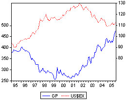
Figure 4 US Nominal Broad Dollar Index and corresponding
Gold Price. (US dollars an ounce)
Figure 4 plots the gold price (Gp) along
with the US dollar index and reveals a strong negative correlation
between the US nominal broad dollar index (US$ex) and the
gold price. Gold has been labelled a hedge to long-run fluctuations
in the US dollar because of the rational economic reasoning
that; when a currency weakens, people lose confidence in fiat
money and therefore switch to gold, as the dollar weakens
we would expect to see a rise in the demand for gold and thus
a rise in the price of gold (Levin and Wright, 2006:37). This
relates closely to the fact that the principal competition
facing gold as a reserve asset is the US dollar; in many instances
Reserve banks choose between holding gold (see Table 1) and
holding US dollars as their reserve asset. A numerical example
from Hussman (1999:1) illustrates this concept. Let’s
assume an exchange rate of R7/$1 and a gold price of $300
an ounce. This would translate into a rand gold price of R2100
an ounce. Now lets assume the value of the dollar (US$ex)
depreciates to R6/$1. This will result in a decrease in the
Rand denominated gold price from R2100 to R1800 an ounce,
(R6 ? $300oz). Thus a depreciation of the dollar will make
the gold price cheaper outside the dollar dominated area and
would result in an increase in the demand for gold, and lift
the US dollar gold price (Hussman, 1999:1). This analysis
supports the findings of Capie Mills and Wood (2004:9), which
state that the gold price has performed as a hedge to fluctuations
in exchange rates.
Figure 4 illustrates the negative relationship
between 1995 and 2004 very clearly. However the negative relationship
breaks down in 2005. Over this period both the gold price
(Gp) and the US nominal broad dollar index (US$ex) increase.
During 2005 a rise in the value of the Broad Nominal dollar
index, which is an indicator of a strong dollar, brought about
a rise in the price of gold.
3.1e. World
Income
Monthly industrial production data for all
developed countries was used as a proxy for world income.
Industrial production is very closely related to world income
due to the strong economic links that exist between; the business
cycle, Gross Domestic Product (GDP), and industrial production.
A large component of GDP is made of industrial production
itself.

Figure 5 World Income and corresponding Gold Price. (US
dollars an ounce)
A positive relationship exists between, income
and the demand for any normal good. This is because with an
increase in income, it is expected that the demand for and
as a result, the price of a good would increase. Similarly
it is rational to expect the same relationship exists in this
analysis. As mentioned in section 3, an expected rise in world
income will induce an increase in the demand for jewellery,
commemorative gold coins, and for gold as an investment good,
and as a consequence, a corresponding rise in the price of
gold.
3.2 Model Specifications
The variables chosen are those which have
displayed empirical and theoretical links with the demand
for gold, and which the author believes are responsible for
driving the gold price for the period January 1995 to November
2005. This paper makes use of the assumption made by Lawrence
(2003) who theorises that the supply of gold is perfectly
elastic. Lawrence theorises that a vast proportion of the
worlds stock of gold is available in a form that can easily
enter the market. Therefore it is unnecessary to express the
variables responsible for the supply of gold. A gold demand
function has been adapted from Ghosh, Levin, Macmillan, and
Wright (2002), and can be expressed as follows:
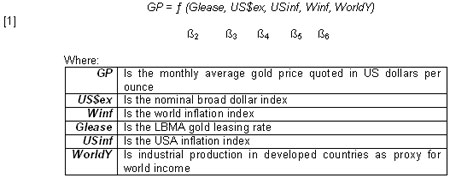
Generally the log-linear model has been used
for most empirical research. It was therefore decided to use
a semilog-linear model and transform the data by taking the
logarithms. The specific nature of the data USinf and Winf
meant that it was not necessary to transform it into the logarithms.
The advantage of this method is the effect of compression
on the scale of each variable and hence a stabilizing of the
variance of the data (Capie Mills and Wood, 2004:13). This
paper can only comment on the relationships between variables
for the specified period January 1995 to November 2005 much
like a snapshot in time. The forecasting capability of this
model is therefore limited.
By denoting the logarithm by symbol; ln,
the following semilog equation can be yielded:

3.2a. Coefficients
and a Priori Expectations
This model hypothesises that the gold price
(dependent variable) can be determined by US and world inflation,
world income, the nominal broad dollar index and the gold
lease rate (independent variables).
The US inflation rate ß4 measures the
responsiveness of gold demand to changes in the US inflation
rate. The general consensus among economists is that gold
tends to move with the inflation rate based on the assumption
that gold is a safe haven and provides investors with protection
against falling purchasing power. It is expected that ß4>0.
Levin and Wright (2006:27) mention that realistically there
is no single measure of inflation that will apply to every
investor. This paper thus includes a measure of world inflation
ß5. Levin and Wright (2006:27) indicate that, the extent
to which the price of gold is determined either by investors
within the US or outside the US is unclear, and thus two measures
of inflation are provided. It can therefore be expected that
ß5>0.
The nominal broad dollar index or ß3,
measures the responsiveness of gold demand to changes in the
strength of the dollar against the currencies of major trading
partners. As the dollar depreciates, the value of gold denominated
in foreign currency falls and it is expected that an increase
in the demand for gold outside the dollar dominated region
will be experienced. Thus, it is expected that ß3<0,
indicating a negative relationship.
The gold lease rate or ß2 can be viewed
according to Levin and Wright (2006:27), as “the opportunity
cost of holding gold.” It is therefore expected that
ß2<0, as the leasing rate increases, ceteris paribus,
the demand for gold will drop. The extent of the relationship
is under question due to the fact that the amount of physical
gold leased is relatively small in comparison to the total
known above ground gold stock piles (see Table 1), which clearly
indicates the accumulated amount of gold leased by central
banks, measured in tonnes.
ß6, is a proxy for world income, and measures the responsiveness
of gold demand to changes in world income. Economic theory
and empirical study suggest that an increase in world income
is expected to induce a rise in the demand for gold, thus
it is expected that ß6>0. The interpretation limitations
of this variable as discussed above must be taken into account
and will result in difficulties in interpreting the relationship.
4. Results
The variables; world income, world inflation, the gold lease
rate, inflation in the US, and the US broad dollar index,
are believed to have a direct impact on the market price of
gold. The econometric results are presented below and provide
an empirical analysis of the variables mentioned, thus providing
a platform for more extensive testing.
4.1 Estimation of a Simple Semi-Log
Regression Model
Thus far, the gold price is assumed to be a function of the
gold lease rate, US dollar index, US inflation, world inflation,
and world income. The results from this estimation are reported
as follows.
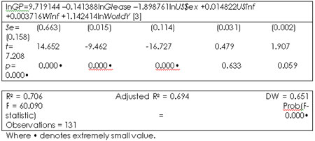
As a measure of how well the expression fits
the data the adjusted R2 is used, which takes into account
the number of explanatory variables, and reveals that approximately
seventy percent of the variation in the gold price can be
explained by the explanatory variables. The Prob(F-statistic)
indicates the statistical significance level at which the
null hypothesis, expressed as the five independent variables
having no impact on the dependent variables, can be rejected.
The F value is significant at the one percent level, the probability
actually being 0.000•, indicating that the null hypothesis
can be rejected.
In considering the significance of variables
individually, each coefficient has the theoretically expected
sign. The results of the coefficients US$ex, WorldY, Glease,
and Winf are attractive. Each supported by a low standard
error and a high t-value, indication that independently, Glease,
US$ex, WorldY coefficients are highly statistically significant
at the one percent level, and Winf at the ten percent level.
The coefficient USinf is disappointing. USinf
is not statistically significant at the ten percent level.
Suggesting that month-to-month inflation in the US does not
have any statistically significant influence on the price
of gold. On the other hand, the inflation coefficient Winf
does show a lower standard error and higher t-value, and is
statistically significant at the six percent level, suggesting
that, Winf is significant as an explanatory variable for the
period January 1995 to November 2005.
There are three possible explanations for
this profound outcome. Why would month-to-month world inflation
be relevant, and month-to-month US inflation not? Firstly,
it supports the view of Ghosh, Levin, Macmillan, and Wright
(2002), who conclude that the influence of inflation on the
gold price can only be viewed in the long-run. Considering
that this investigation extends over a relatively short period
of time(12) , we may not expect to capture
the full influence of inflation as an explanatory variable
both world wide and within the USA. Secondly, it can be interpreted
that for the period under investigation, investors outside
the US, buying gold denominated in a currency other than the
US dollar, for the purposes of being an inflation hedge, influences
the gold price more than investors buying gold for the same
purposes, within the USA. Thirdly, the variable USinf may
not be statistically significant due to the problem of multicollinearity
in the model.
The Granger Causality Test can be used to
test whether each explanatory variable considered individually,
during the period under investigation, was the “cause”
of fluctuations in the gold price. The results were as follows:
the null hypothesis in each case indicates that individually
the independent variable do not “Granger-cause”
the gold price. The test applies to a very specific concept
of causality known as Granger-causality. Note that the best
discussion concerning causality is economic theory itself,
which was discussed in section 3.
Table 2. Pairwise Granger Causality Test
| |
F - value |
P - value |
ln(Glease) does not cause ln(GP) |
6.88 |
0.01 |
ln(US$ex) does not cause ln(GP) |
4.95 |
0.03 |
USinf does not cause ln(GP) |
0.75 |
0.38 |
Winf does not causer ln(GP) |
0.32 |
0.56 |
ln(WorldY) does not cause ln(GP) |
0.06 |
0.79 |
The F value for Glease and US$ex are significant
at the three percent level of significance. It is possible
to reject the null hypothesis and conclude that the direction
of causality runs from the gold lease rate to the gold price
and from the US broad dollar index to the gold price. This
result conforms to priori expectations. On the other hand,
it is not possible to reject the null hypothesis that US inflation,
world inflation, and world income do not cause the gold price
(Gujarati, 2003:696). The test was conducted at one lag. This
decision was based on the fact that the major trading houses
around the world are now equipped to follow the market on
a twenty-four hour basis and so, as the earth turns the price
of gold follows the sun. In such a well organised highly liquid
and deep market, it can be expected that any change in factors
believed to influence the gold price, would be felt after
a short lag period via a change in the price of gold (Kettell,
203:19820).
Before going any further, more shortfalls
of the investigation should be revealed. There is cause to
believe that the results of the estimated model may be spurious.
Firstly, as a good rule of thumb, Granger and Newbold, 1974
in Gujarati, (2003:823), suggest that an R2 greater than DW
is a reliable indicator to suggest that an estimated regression
may be spurious. Multicollenearity and autocorrelation problems
may have affected the results due to the low DW statistic.
Problems emerge in using time series data to estimate a regression
when data is found to be non-stationary, as mentioned at the
beginning of section 4.
4.1a. Stationary
Test
The results of the Augmented Dickey-Fuller
Test (ADF) are reported in Table 4. The testing of time series
data does however pose challenges. According to Gujarati (2003:798),
a time series is stationary when it’s mean, variance
and auto covariance remain constant at all time periods. If
a time series is non-stationary its behaviour can only be
studied for the specific time period under investigation.
Each time series set will be for a specific period, and it
will not be possible to generalise it to other time periods
and hence will have little practical forecasting value. The
test for stationary time series data was performed up to second
difference where necessary. The process involves testing the
ADF-statistic corresponding with each significant t-statistic.
After testing for a unit root the results reveal that some
variables did contain a unit root and are therefore non-stationary.
The estimated model may not be reliable and hence any further
conclusions deduced should be taken with a grain of salt.
It is important to note that the ADF test
is regarded as the most efficient among the available simple
tests for stationarity.
Table 4. Unit Root Test
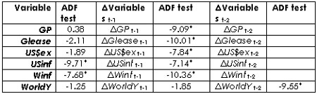
Note: * indicates that the variable under consideration is
stationary at the 1 percent level,
** indicates that the variable under consideration is stationary
at the 5 percent level
Results reveal that at level, the USinf and
Winf time series are stationary. The time series for the GP,
Glease and US$ex become stationary at their first difference.
However, at first difference, the time series WorldY remains
non-stationary. It is only after performing the ADF test at
the second difference that the series WorldY is made stationary
at the one percent level of significance. It is important
to state the limitations of the ADF test. The ADF test has
“low power” that is, the test may find a unit
root even when none exists (Gujarati, 2003:819). As an alternative
the Phillips-Perron (pp) Unit Root Test can be adopted.
In normal circumstances, a regression equation
which makes use of time series data that is found to be non-stationary,
will deliver results that may be spurious. A procedure known
as the Engle-Granger (1987) error correction technique could
then be applied. Testing for co-integrated variables involves
estimating a co-integrating vector. In simple terms, this
vector can be interpreted as the co-integrating long-run relationship
between the variables and is very important in determining
the ability of a model to be used in forecasting activities.
4.2 Analysis
of Long Run Relationship
As a quicker and relatively simpler means of establishing
a long-run relationship between the gold price and the explanatory
variables, this paper employs the Co-integrating Regression
Durbin-Watson Test.
Table 5.Co-integrating Regression Durbin-Watson
Test (CRDW).
| DW = 0.651 |
| Test critical values: |
| 1% level |
0.511 |
| 5% level |
0.386 |
10% level
|
0.322 |
The Durbin-Watson value is obtained from
the regression. The CRDW test involves testing the null hypothesis
that the regression is co-integrated. In this case the DW
is greater than the critical value of 0.511, which indicates
we can not reject the null hypothesis that the regression
is co-integrated. This suggests that the regression ln(GP)
and ln(Glease), ln(US$ex), USinf, Winf, ln(WorldY), is co-integrated
at a one percent level of significance. It can therefore be
concluded that although the variables individually do display
random walks, there does seem to be evidence of a stable long
run relationship between them (Gujarati 2003:824). For a more
robust test the Johansen procedure is recommended.
5. Summary
and Conclusion
Table 6. Summary of SemiLog-linear model
results.

Note: * indicates coefficient is significance at the 1 percent
level,
** indicates coefficient is significance at the 5 percent
level,
*** indicates coefficient is significance at the 10 percent
level.
The first conclusion and a relatively obvious
one, is the existence of a highly statistically significant
negative relationship between changes in the strength of the
US dollar against a basket of currencies and changes in the
gold price. Using the Pairwise Granger Causality Test as illustrated
in Table 2, we may further conclude that an appreciation in
the US dollar index by 1% causes the gold price to fall by
approximately 1.899%. Similarly, 1% depreciation in the dollar
against major currencies causes the price of gold to rise
approximately 1.899%.
The second conclusion is that there exists
a statistically significant negative relationship between
the gold lease rate and the gold price. The Granger Causality
test confirms a priori expectations that a positive change
in the gold lease rate does “Granger Causes” a
negative change in the gold price. The model suggests that
a 1% increase in the gold lease rate causes the price of gold
to fall approximately 0.141%.
The third conclusion, world income did play
an important role in determining the gold price over the period
January 1995 to November 2005. A 1% increase in world income
results in approximately a 1.142% rise in the gold price.
The relationship conforms to priori expectations; however
the test in Table 2 reveals that causality between world income
and the gold price can not be established. Two alternative
explanations can be given for this; it is possible that monthly
industrial production data for all developed countries has
not performed well as a proxy for world income. As a second
alternative, it is possible that the time frame limitations
do not take into account any long run relationship. If this
were the case, an investigation of this nature would not be
able to quantify the true long run relationship accurately.
Fourth it can be concluded that Gold’s
expected relation with inflation was inconclusive over the
same period. The analysis failed to locate a conclusive statistical
relationship between changes in the gold price and changes
in US inflation. The semilog-linear model does suggest that
a 1% increase in US inflation and world inflation causes the
gold price to rise by approximately 1.482% and 0.372% respectively.
This paper does however find a statistically significant positive
relation with world inflation and the price of gold. These
thought provoking findings concerning the general relationship
between inflation and gold reveal that the impact in the gold
market by participants, as a whole, outside the USA are of
greater influence and significance that investors within the
USA.
5.1 Limitations
of Study and Further Research.
The major short coming of the empirical findings
is the inability of this paper to effectively deal with the
problem of non-stationary time series data.
To reiterate the famous words once said by
Faugère and Van Erlach (2005:3), “assessing the
fair value of gold largely remains a mystery in finance.”
This paper through simple empirical analysis has revealed
results consistent with popular belief concerning the variables
responsible for driving the gold price as well as their respective
relationships. The scope of this investigation has been limited
to include only variables believed to be the major movers
in the gold market and where data was available. These limitations
leave room for useful future research taking into account
such variables not included in this paper as Central Bank
official buying and selling in bullion, producer hedging activities
like forward selling of expected production, a simple gold
supply and demand analysis including industrial and jewellery
demand for gold, the effect of world terrorism and uncertainty
caused by political and financial risk. It has been suggested
that global speculative activities may also account for a
significant proportion of gold price fluctuations. The result
of rapid economic growth and expansion in China and India
has certainly lead to an increase in the demand for natural
resources and mineral commodities at a furious pace and lead
to an increase in the demand for gold is Asia. The exact extent
of this “Central Asian” influence on the gold
market is unknown and there is a need for further detailed
research.
FOOT
NOTES
(1) Department of Economics and Economic
History, Rhodes University. The author wishes to thank Andrew
Sullivan and Jessica Cross (CEO) of Virtual Metals Research
and Consultancy, London; and Ted Reeve of Haliburton Mineral
Services, Toronto; for providing daily gold lease rates. The
assistance of Roger Baxter, the South African Chamber of Mines
Chief Economist, for providing the GFMS Global Hedging Book
Analysis, Q4-2005 is here by acknowledged, as well as MJ Aziakpono
a Senior Lecture, Department of Economics, Rhodes University
for providing IMF World Inflation and Industrial production
data. The input advice and assistance of Magda Kasyoka Wilson,
a senior lecture, Department of Economics Rhodes University,
is duly noted.
Conclusions derived are those exclusively of the author.
(2) Containing or impregnated with minerals: a mineral deposit.
(3) Gold bars.
(4) Between mid 1980’s and early 2001.
(5) Gold is being examined in its capacity as a financial
asset, in terms of its role as a portfolio diversifier and
therefore, the phrase “returns on gold” can be
likened to the return on stocks and bonds.
(6) 31.103 Grams; 408.6 Grains; 1.097 Oz Avoirdupois; 20 Pennyweights.
(7) Month-to-month inflation formula = (CPI(1995:02) –
CPI(1995:01) / CPI(1995:01))*100
(8) The author wishes to thank Mr MJ Aziakpono a Senior Lecture,
Department of Economics, Rhodes University for the unpaid
assistance and helpful suggestion.
(9) The time series data set included the 1 month; 3month;
6 month and 12 month daily lease rate from 1 January 1995
– 2 May 2006.
(10) Consisting of 19 internationally traded commodities,
including gold.
(11) ($550/oz. × 16 oz. /lb. × 2,000lbs. / ton
× 31,445 tons) × (R7.7 : $1)
(12) Ten years and eleven months
REFERENCES
CAPIE, F., MILLS, T.C and
WOOD, G., 2004. Gold as a Hedge against the US Dollar. World
Gold Council. No. 30, September.
DEPARTMENT OF MINERALS AND ENERGY, 2004. South Africa’s
Mineral Industry 2003/2004. Pretoria: The DME.
DEVARAJAN, S. and FISHER, A., 1981. Hotelling’s “Economics
of Exhaustible Resources” Fifty Years Later. Journal
of Economic Literature. Vol.?I? (March 1981), pp. 65 –
73.
DORSCH, G., 2006. The “Commodity Super Cycle”
How long can it last? [Online]. Available: http://www.gold-eagle.com/editorials_05/dorsch021306.html.
[Accessed 2 March 2006]
THE FREE DICTIONARY., 2006. mineralized. [Online]. Available:
http://www.thefreedictionary.com/mineralized. [Accessed 21
September 2006].
EVANS, D., 2004. Why Invest in Gold Now? [Online]. Avaliable:
http://www.ctgold.com.au/downloadablefiles/why%20Invest%20In%20gold%20now.pdf.
[Accessed 22 February 2006].
FAUGÈRE, C. and VAN ERLACH, J., 2005. The Price of
Gold: A Global Required Yield Theory. Journal of Investing.
14, 1: 99 – 111.
GHOSH, D., LEVIN, E.J., MACMILLAN, P. and WRIGHT, R.E., 2002.
Gold as an Inflation Hedge? Studies in Economics and Finance.
22, 1: 1 – 25.
GUJARATI, P.,2003. Basic Econometrics (5e). Chicago. USA.
McGraw Hill.
GOLD FIELDS MINERAL SERVICES LTD, 2006. Global Hedge Book
Analysis Q4-2005. London, Regent Street Hedges House: GFMS.
GOLD FIELDS MINERAL SERVICES LTD, 1991. Gold 1991. London
Greencoat House: GFMS.
GOLDORG, 2006. Gold Jewelry in China. [Online]. Available:
http://goldprice.org/gold-jewelry/2006/01/gold-jewelry-in-china.html.
[Accessed 20 March 2006]
HUSSMAN, J.P., 2000. Four simple indicators for monitoring
the condition of the precious metals markets. [Online]. Available:
http://www.hussmanfunds.com/html/gold.htm. [Accessed 3 March
2006].
KETTELL, B., 1982. Gold. Harvard Square Cambridge: Ballinger
Publishing Company.
KEYFITZ, R., 2004. Currencies and commodities: modeling the
impact of exchange rates on commodity prices in the world
market. IMF staff papers. 41: 236 – 261.
LAWRENCE, C., 2003. Why is gold different from other assets?
An empirical investigation. World Gold Council. [Online].
Available: http://www.gold.org/value/stats/research/pdf/C%20Lawrence.pdf.
[Accessed 1 March 2006].
LEVIN, E.J and WRIGHT, R.E., 2006. Short-run and Long-run
Determination of the Price of Gold. World Gold Council. No.
32, June.
MUSCATELLI, V.A and HURN, S., 1992. Cointegration and Dynamic
Time Series Models. Journal of Economic Surveys. 6, 1: 1 –
38.
RYAN, B., 2006. So far, so good….UpFront. January. Pp78-79.
SALANT, S.W., 1995. The Economics Of Natural Resource Extraction:
A Primer For Development Economists. The World Bank Research
Observer. 10, 1: 93 – 111.
STAASTAD, L. and SCAACCIAVILLANI, F., 1996.The price of gold
and the exchange rate. Journal of International Money and
Finance. 15, 6: 879 – 897.
VIRTUAL METALS RESEARCH AND CONSULTENCY., 2005. The Yellow
Book. London.
WAGGONER, J., 2005. Gold price glitters, but gather nuggets
of data before buying. USA Today. 2 December. pp4. [Online].
Available:http://search.epnet.com/login.aspx?direct=true&db=aph&an=J0E000426560905.
|


